A notebook on the Extended Kalman Filter

What to consider before diving into this post

If you have reached this post after googling how to start studying the SLAM problem and the Kalman Filter, up to this moment you might have found two kinds of sources of information:

Very basic explanations but purely theoretical. You might be asking yourself: Ok, I got the basis, but what do I do know? I don’t know where to start!
Not purely theoretical approaches, but too advanced for your current level.

When I found myself in this situation, I found a missing 1.2 point that helped me going from 1. to 2. So if you are in this situation, here is my recommendation:

First, the theory

First, go watch the Cyrill Stachniss course on youtube. He has a very popular course from 2013 in his channel, and all the videos are really good, but recently he has uploaded new versions of those videos that I find even better. He gives simple examples, closely related to the code, that make it much more clear to understand.

However, if you still find this course too advanced, the course from Claus Brenner, also on Youtube, could be a better start for you. But if you already know some concepts on Bayesian probability, the Cyrill course shoul be easy for you to get.

Now, start coding

Probability is the permanently underestimated and forgotten field in mathematics, or at least that’s my experience from studying engineering. Kalman filters are based in Bayesian filters, and I recommend you to do a quick review on all them, from the mathematics point of view, before getting into robotics. I found a gem for that in the internet, which is this notebook by Roger Labbe. It is really amazing. It meets a perfect balance between theory and examples, and you can execute the code in your notebook and play with it!

After that, the next step is applying the actual Kalman filter to a more “robotic” example. Here, we get back to Cyrill course. It has some code resources for the theoretical course. However, they are programmed in Octave, some sort of open-source matlab. Personally, I’m not very much into Octave… and that’s where this post arised! I have adapted the Octave functions from Cyrill’s course to Python, and I have executed them in a Jupyter notebook for the sake of clarity.

Here, you will find a combination of theory and code. But, as the title states, it is just a notebook. It is meant for someone that is somewhat familiar with Kalman filters, and is more a review notebook to refresh concepts than a studying notebook. It doesn’t contain all the code, neither all the theory. The Jupyter notebook is submitted on my github for you to execute. And if you need to clarify better the theory concepts, I recommend you to go to any of the previous sources I mentioned. In this post, only the most important functions and concepts are included.

First, I will briefly mention the Kalman filter, which is the most basic algorithm and that nowadays is not deployed into any real robot, but still very convenient to study as a basis to the subsequent algorithms. And then, we will get hands-on into the Extended Kalman Filter, one of the most (if not the most) popular versions of the Kalman filter.

The Kalman Filter

This filter is the optimal estimator for linear functions and Gaussian distributions. The Kalman filter can be used as a solution to the online SLAM problem, defined as follows:

Given:

The robot’s controls $u_{1:T} = {u_1,u_2,u_3...,u_T}$
Observations $z_{1:T} = {z_1,z_2,z_3...,z_T}$

Wanted:

Map of the environment $m$
Path of the robot $x_{0:T} = {x_0,x_1,x_2...,x_T}$

We will make a probabilistic estimation of the robot’s path and the map according to the motion and observation models.

Motion Model

The motion model describes the relative motion of the robot. Some examples of motion model are the Odometry-based model (wheeled robots) or the velocity-based model (flying robots).

The motion model is represented by matrices and thus is a linear function.

$x_t = A_tx_{t-1} + B_tu_t + \epsilon_t$

$A_t (n\times n)$ maps the state at $t$, given the previous state at $t-1$.
$B_t (n\times l)$ describes state change from $t-1$ to $t$ , given control command.

Observation Model

The observation or sensor model relates measurements with the robot’s pose: what I am going to observe given that I know the pose or the map. The Beam-Endpoint model is characterized by a gaussian blur around the obstables. The Ray-cast model experiments an exponential decay and covers dynamic obstacles.

The linear mapping between the state and the observation space:

$z_t = C_tx_{t} + \delta_t$

$C_t (k\times n)$ maps state $x_t$ to an observation $z_t$ .

The Kalman filter is a recursive algorithm and it is computed as follows:

Where $Q_t$ and $R_t$ describe measurement and motion noise, $\mathbf{\mu}_{t}$ is the mean, $\textstyle\sum_t$ is the covariance (uncertainty), $K_t$ is the Kalman gain. The Kalman gain computes how certain I am about the prediction with respect to the motion.

We introduce to the algorithm our current estimate of where we have been in tearms of mean estimate and covariance matrix, as well as the new control command and the observations. We want to update the mean and the covariance matrix so we transit from t-1 to t. We are computing a weighted sum with the Kalman gain weighting the prediction and the correction.

The Extended Kalman Filter

However, in most real scenarios we do not have linear functions to describe the movements or the sensor model. Non-linear functions lead to non-Gaussian distributions and we cannot use the Kalman filter anymore. This is resolved by the Extended Kalman Filter by local linearization. However, we’re still assuming Gaussian noise and Gaussian uncertainties.

The algorithm for the Extended Kalman Filter is:

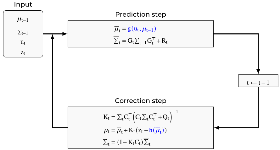
The terms highlighted in blue are those in which the EKF perform the local linearization. Hereafter, I will introduce how these terms are computed.

Using the EKF to solve the SLAM problem

First we need to define our state vector, and the assumptions for the example that we are using in this notebook:

Assumption: known correspondences. That is, when I get an observation, I know which landmark it is in my map.
State space (for 2D plane) contains the robot pose (3 dimensions) and the landmark locations (2 dimensions each), and it’s defined as:

$x_t = ( \underbrace{x,y,\theta}_{\text{robot's pose}},\underbrace{m_{1,x},m_{1,y}}_{\text{landmark 1}},...,\underbrace{m_{n,x},m_{n,y}}_{\text{landmark n}})^T$

State representation (very compactly, with $x_R\rightarrow x)$ ):

$\underbrace{\begin{pmatrix}x\\m\end{pmatrix}}_{\mu}\underbrace{\begin{pmatrix}\textstyle\sum_{xx} \textstyle\sum_{xm}\\\textstyle\sum_{mx} \textstyle\sum_{mm}\end{pmatrix}}_{\textstyle\sum}$

With $\sum_{xx}$ representing the uncertainty around the pose, $\sum_{mm}$ the uncertainty about the landmark location, and $\sum_{xm}$ the link between the landmark locations and the position of the robot within the platform.

Prediction step: defining g

In this step we only update the pose of the robot $x,y,\theta$ and its covariance $\sum_{xx}$ according to the motion model $g$ . Note that since we are just considering the robot’s movement, without taking into account the sensor’s measurements yet, the landmarks locations are not updated in this step.

The motion model

Here the motion model considered is the Odometry Model:

The robot moves from $xytheta$ to $xythetaprima$
We have odometry information $u$

$\delta_{trans} = \sqrt{(\overline{x}'-\overline{x})^2+(\overline{y}'-\overline{y})^2}$

$\delta_{rot1} = atan2(\overline{y}'-\overline{y},\overline{x}'-\overline{x})-\overline{\theta}$

$\delta_{rot2} = \overline{\theta}'-\overline{\theta}-\delta_{rot1}$

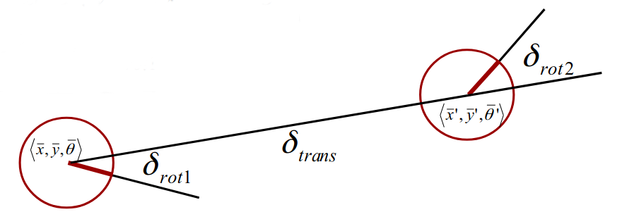
Thus, our odometry motion model (without the noise model) that we will use to update the robot pose in the state vector $\mu$ is:

$x' = x + \delta_{trans}\cos{(\theta+\delta_{rot1})}$

$y' = y + \delta_{trans}\sin{(\theta+\delta_{rot1})}$

$\theta' = \theta + \delta_{rot1} + \delta_{rot2}$

Next, we update the elements in the covariance matrix associated to the robot pose by performing a local linearization of the function. This is achieved with the partial derivatives of the previous functions, that is, with the Jacobian matrix $G$ .

$G_t^x = \frac{\delta g(u_t,\mu')}{\delta (x,y,\theta)}$

Remember that we’re only updating the robot values in the state space. That is, our Jacobian will have the structure:

$G_t = \begin{bmatrix} \frac{\delta g(u_t,\mu')}{\delta (x,y,\theta)} & \textbf{0}\\ \textbf{0} & \textbf{I} \end{bmatrix}$

def prediction_step( mu, sigma, u):
    ''' Updates the belief concerning the robot pose according to the motion model,
    args:
    - mu :: 2N+3 x 1 vector representing the state mean.
    - sigma :: 2N+3 x 2N+3 covariance matrix.
    - u: odometry reading (r1, t, r2).    

    '''
    m,n = sigma.shape

    # Compute new mu based on the noise-free (odometry-based) motion model
    mu[0,0] = mu[0,0] + data['t'][0] * np.cos(mu[2,0] + data['r1'][0]) # x
    mu[1,0] = mu[1,0] + data['t'][0] * np.sin(mu[2,0] + data['r1'][0]) # y
    mu[2,0] = mu[2,0] + data['r1'][0] + data['r2'][0] # y
    mu[2,0] = normalize_angle(mu[2,0])

    # Compute the 3x3 Jacobian Gx of the motion model
    Gx = np.identity(3)
    Gx[0,2] = - data['t'][0] * np.sin(mu[2,0] + data['r1'][0])
    Gx[1,2] =   data['t'][0] * np.cos(mu[2,0] + data['r1'][0])

    # Construct the full Jacobian G
    G = np.concatenate((Gx,np.zeros((3,n-3))),axis = 1)
    aux = np.concatenate((np.zeros((n-3,3)), np.identity(n-3)),axis = 1)
    G = np.concatenate((G,aux), axis = 0)

    # Motion noise R
    motionNoise = 0.1
    R3 = np.identity(3)*motionNoise
    R3[2,2] = motionNoise/10

    R = np.zeros((sigma.shape))

    R[0:3, 0:3] = R3

    # Compute predicted sigma
    sigma = np.matmul(G,np.matmul(sigma,G.T)) +R # i.e.  sigma = G*sigma*G.T + R


    return mu,sigma

Correction step

Once the pose has been update, it’s time for the correction.

Predicted measurement $h(x)$ : we need to predict what the robot sees. For that, we take the current position of the robot, and the position of the landmarks in the map, and with that we compute our predicted measurement.
Obtained measurement $z$ : we take the real observations of the landmarks according to the sensor.
Data association: we compute the discrepancy between $h(x)$ and $z$ .
Update step: finally, all the elements in $\mu$ and $\sum$ are updated

def correction_step(mu,sigma,z,observedLandmarks):
    ''' Updates the belief, i. e., mu and sigma after observing landmarks, according to the sensor model.
        The employed sensor model measures the range and bearing of a landmark.
        mu: 2N+3 x 1 vector representing the state mean.
        The first 3 components of mu correspond to the current estimate of the robot pose [x; y; theta]
        The current pose estimate of the landmark with id = j is: [mu(2*j+2); mu(2*j+3)]
        sigma: 2N+3 x 2N+3 is the covariance matrix
        z: struct array containing the landmark observations.
        Each observation z(i) has an id z(i).id, a range z(i).range, and a bearing z(i).bearing
        The vector observedLandmarks indicates which landmarks have been observed at some point by the robot.
        observedLandmarks(j) is false if the landmark with id = j has never been observed before.
    '''
    # Number of measurements in this time step
    m = z.shape[0]
    # Number of dimensions to mu
    dim = mu.shape[0]
    # Z: vectorized form of all measurements made in this time step: [range_1; bearing_1; range_2; bearing_2; ...; range_m; bearing_m]
    # ExpectedZ: vectorized form of all expected measurements in the same form.
    # They are initialized here and should be filled out in the for loop below
    Z = np.zeros([m*2, 1],float)
    expectedZ = np.zeros([m*2, 1],float)

    # Iterate over the measurements and compute the H matrix
    # (stacked Jacobian blocks of the measurement function)
    # H will be 2m x 2N+3
    H = []

    j = 0
    for i,row in z.iterrows():
        # Get the id of the landmark corresponding to the i-th observation
        landmarkId = int(row['r1']) # r1 == ID here
        #landmarkId = landmarkId -1 # adapt the 1-9 range to 0-8 range of the array

        # If the landmark is obeserved for the first time:
        if (observedLandmarks[0][landmarkId-1] == 0):
            # Initialize its pose in mu based on the measurement and the current robot pose:
            a = float(row['t']*np.cos(row['r2']+mu[2]))
            b = float(row['t']*np.sin(row['r2']+mu[2]))
            mu[2*landmarkId+1 : 2*landmarkId+3] = mu[0:2] + np.array([[a], [b]])

            # Indicate in the observedLandmarks vector that this landmark has been observed
            observedLandmarks[0][landmarkId-1] = 1  

        # Add the landmark measurement to the Z vector   
        Z[2*j] = row['t']
        Z[2*j+1] = row['r2']

        # Use the current estimate of the landmark pose
        # to compute the corresponding expected measurement in expectedZ:
        delta = mu[2 * landmarkId + 1 : 2 * landmarkId + 2+1] - mu[0:2]
        q = np.matmul(delta.T,delta)

        expectedZ[2*j] = math.sqrt(q)
        expectedZ[2*j+1] = normalize_angle(np.arctan2(delta[1],delta[0]) - mu[2])      

        delta0 = float(delta[0])
        delta1 = float(delta[1])

        # Compute the Jacobian Hi of the measurement function h for this observation
        Hi = 1/q * np.array([[float(-math.sqrt(q)*delta0),-math.sqrt(q)*delta1, 0, math.sqrt(q)*delta0, math.sqrt(q)*delta1], [ delta1, -delta0, float(-q), -delta1, delta0] ])

        # Map Jacobian Hi to high dimensional space by a mapping matrix Fxj
        Fxj = np.zeros([5,dim])
        Fxj[0:3,0:3] = np.identity(3)
        Fxj[3,2*landmarkId+1] = 1
        Fxj[4,2*landmarkId+2] = 1

        Hi = np.matmul(Hi, Fxj)


        # Augment H with the new Hi     

        H.append(Hi)

        j+=1



    # Construct the sensor noise matrix Q
    Q = 0.01*np.identity(2*m)

    # Compute the Kalman gain
    # K = sigma * H.T * inv(H * sigma * H.T + Q)
    Hnp = np.asarray(H).reshape((2*m,dim))
    sigmaxHt = np.matmul(sigma,Hnp.T)
    inverse = np.linalg.inv(np.matmul(Hnp,sigmaxHt)+Q)    
    K = np.matmul(sigmaxHt,inverse)

    # Compute the difference between the expected and recorded measurements.
    # Remember to normalize the bearings after subtracting!

    diffZ = normalize_all_bearings(Z-expectedZ)

    # Finish the correction step by computing the new mu and sigma.
    # Normalize theta in the robot pose.
    mu = mu + np.matmul(K, diffZ)
    # sigma = (eye(dim) - K * H) * sigma
    sigma = np.matmul((np.identity(dim) - np.matmul(K, Hnp)), sigma)

    return mu, sigma, observedLandmarks

Initializing the belief

Given that we know the number of landmarks in our map, we can define the shape of the mean and the covariance matrix:

mu: 2N+3x1 vector representing the mean of the normal distribution. The first 3 components of mu correspond to the pose of the robot, and the landmark poses (xi, yi) are stacked in ascending id order.
sigma: (2N+3)x(2N+3) covariance matrix of the normal distribution.

Everything is completely unknown in the beginnig, so we define the starting point as our coordinate system. That is, $\mu = \textbf{0}$ . Since we are completely certain about that (because we’ve defined it), the corresponding values in sigma are also zero $\sum_{xx} = \textbf{0}$ . However, we don’t know anything about the landmarks, because we haven’t seen anything yet, so they have an infinite uncertainty.

# Initialize mu
mu = np.zeros((2*N+3,1),dtype = 'float')
# Initialize sigma
robSigma = np.zeros((3,3))
robMapSigma = np.zeros((3,2*N))
mapSigma = np.identity((2*N))*1000 # 1000 as a "infinite" or just "high" value

aux1 = np.concatenate((robSigma,robMapSigma),axis = 1)
aux2 = np.concatenate((robMapSigma.T,mapSigma), axis = 1)

sigma = np.concatenate((aux1,aux2),axis = 0)

The sigma values corresponding to the robot pose, as mentioned, have 0. value (no uncertainty)

sigma[0:3, 0:3]

array([[0., 0., 0.],
       [0., 0., 0.],
       [0., 0., 0.]])

However, the covariance associated to the landmark pose has infinite value(here 1000, just a high value), for instance, for the first landmark:

sigma[3,3]

1000.0

The EKF loop

Up to this point we have everything ready to execute the Extended Kalman Filter loop in our 2D environment and see what happens. Each element in the map is displayed altogether with the uncertainty of the measurement, plotted as an ellipse. You can see in the video, that the more a landmark is seen by the robot, the smaller the ellipse gets (and thus, the uncertainty).

def ekf_loop(mu,sigma,observedLandmarks,fig,ax,camera):

    for t in range (0,timestepindex[-1]):
        # Perform the prediction step of the EKF
        mu,sigma = prediction_step(mu, sigma, data.loc[(data['timestep'] == t) & (data['sensor'] == 'ODOMETRY')])


        #Perform the correction step of the EKF
        mu, sigma, observedLandmarks = correction_step(mu,sigma,data.loc[(data['timestep'] == t) & (data['sensor'] == 'SENSOR')],observedLandmarks)
        # Generate visualization plots
        fig = plot_state(mu,sigma,world_ldmrks,t,observedLandmarks,data.loc[(data['timestep'] == t) & (data['sensor'] == 'SENSOR')],fig,ax)
        camera.snap()
    return camera, mu[0:3],sigma[0:3,0:3]

observedLandmarks = np.zeros((1,N))
robSigma = np.zeros((3,3))
robMapSigma = np.zeros((3,2*N))
mapSigma = np.identity((2*N))*1000 # 1000 as a "infinite" or just "high" value
aux1 = np.concatenate((robSigma,robMapSigma),axis = 1)
aux2 = np.concatenate((robMapSigma.T,mapSigma), axis = 1)
sigma = np.concatenate((aux1,aux2),axis = 0)
mu = np.zeros((2*9+3,1),dtype = 'float')

fig,ax = plt.subplots()
camera = Camera(fig)

camera = ekf_loop(mu,sigma,observedLandmarks,fig,ax,camera)[0]

animation = camera.animate()
HTML(animation.to_html5_video())       

png

13 May 2021

« To enhance or not to enhance? Computer Vision in challenging imaging conditions

creating ROS metapackages »

Olaya Alvarez-Tuñon Follow
Hi, I am Olaya.

Olaya Alvarez-Tuñon

A notebook on the Extended Kalman Filter

What to consider before diving into this post

The Kalman Filter

The Extended Kalman Filter

Using the EKF to solve the SLAM problem

Prediction step: defining g

The motion model

Correction step

Initializing the belief

The EKF loop

Search

Newsletter

Useful Links

Newsletter for Developers

Connect with me